
Abstract
Write the equations once. Then compile, differentiate, and close the loop.
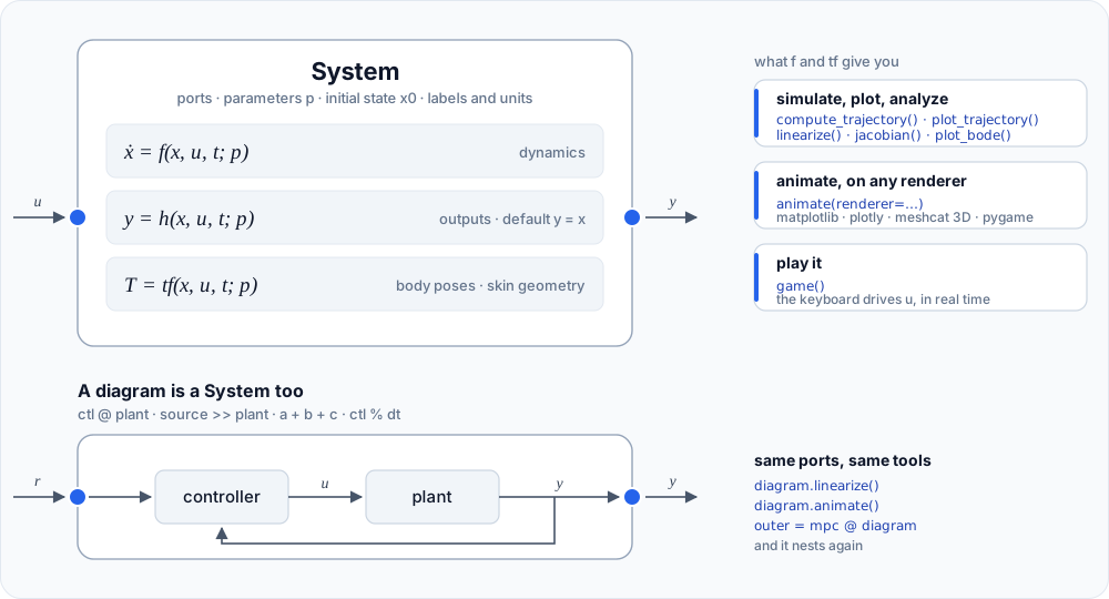
You write a custom dynamical system in ordinary Python — f reads like the textbook.
Diagrams of those systems (ctl @ plant, sources) flatten to one
f. That same graph is JIT-compiled and autodifferentiated under JAX: exact
∂f/∂x, ∂f/∂u, ∂f/∂p, gradients through a rollout, batches of plants or parameters.
That is what makes modern control, fast trajectory optimization, model predictive control, and learning practical on the model you actually wrote. Minilink is the successor of Pyro.
Custom systems, arbitrary diagrams
A model is three functions of the state x, the input u, the time
t and the parameters p:
dx/dt = f(x, u, t; p) ·
y = h(x, u, t; p) ·
T = tf(x, u, t; p)
There is no hidden state on the object. That one convention is what lets a model compose into
diagrams, run in batches and differentiate later. A diagram flattens to one state vector and one
f, so a closed loop linearizes and nests like a plant.
Compile, autodiff, JAX
The same f traces under JAX. One evaluator gives exact derivatives, batched rollouts
and gradients through a whole simulation:
Measured in the showcase notebook on an Apple M4 Max: 1000 rollouts of 1000 RK4 steps take 27 ms as a compiled batch and about 32 s one step at a time in Python. Derivatives are exact to machine precision.
What that unlocks on the plant you wrote:
- modern control on a compiled diagram
- fast trajectory optimization — exact defects, jitted residuals
- MPC that re-solves the same program at the control rate
- learning on the model — gain tuning, identification, neural controllers, RL
Publications & Resources
Project Media
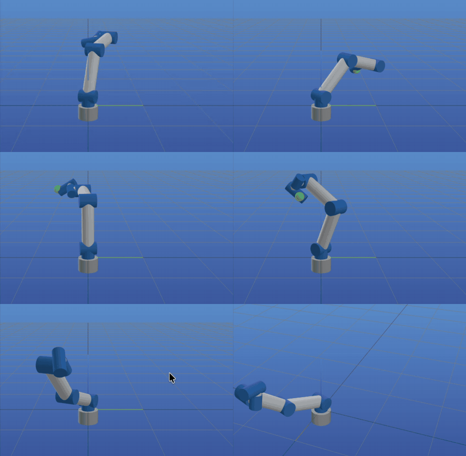
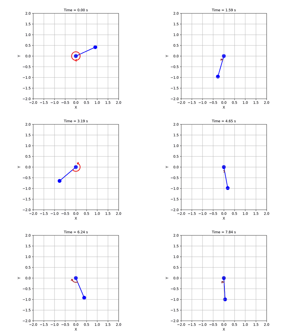
ImpedanceController() @ Pendulum()